The Political Physicist

Note: I wrote this guide for the Saint Mary’s University Astronomy and Physics Society to go along with a tutorial that I will present on the Fortran programming language. I thought I’d post it here in addition to the SMUAPS website.

Fortran, which stands for FORmula TRANslator, is the oldest high level programming language and remains, albeit with significant improvements, one of the main languages used by physicists.¹ Most computational physics is done using Fortran and this is the language typically used in SMU’s Computational Methods for Physicists class. This introduction will show you how to use various useful features of the language in its modern form.² It will do this by defining a problem which we wish a program to solve and then showing how to write such a program. The program can be downloaded here if you want to follow along (which I’d recommend doing). I assume that you already know how the basics of computer programming but have not previously done scientific computing or worked with Fotran. Of course, this will only be a taste of Fortran’s abilities and there will be many features, both simple and complex, which I will not be able to mention. For a good overview of them, see this Wikipedia article.

Table of Contents

• The Problem
  • The Numerical Method
  • Statistics
• The Algorithm
• A Note on Style
• Comments and White Space
• Fortran Basics
  • Basic Program Structure
  • Variables
  • Conditional Statements
  • Loops
• Getting Instructions from the User
• Reading and Writing Data
• Procedures
  • Pass by Reference
  • Functions
  • Subroutines
• Array Syntax
• Compiling and Running Your Program
• Packaging Your Procedures
• Summing Up
• Useful Resources

The Problem

Say we’ve measure the electric potentials at various points in one dimension. We have recorded the location at which the measurement was taken and the value of the potential in a file on our computer. We now want to calculate the electric field that exists at each point where we took a measurement. These results will be printed to a second text file on the computer. The program should also find the average electric field and the standard deviation.

The Numerical Method

To do this, we need to recall that

In our simple, one dimensional case, this becomes

However, we don’t actually know the function \(V(x)\), only the value of \(V\) at particular values of \(x\). So, how do we calculate the derivative? In reality, we’ll have to estimate it. The limit definition of the derivative says

so you might be tempted to use

However, that is only accounting for the rate of change on one side of your data-point, \(i\). Thus, it would be better to use

Of course, this won’t work at two ends of the data set, so in those cases we’ll simply have to make do with half of the information and use something along the lines of our first guess of how to take the derivative.

Statistics

As I hope everyone will know, the average value of some data is given by

As a reminder, the standard deviation of a data-set is

The Algorithm

The basic structure of our program will be as follows

1. Determine the files from which to read and to which to write data.
2. Read the data from the input file.
3. Take the derivative of the data and multiply by negative one.
4. Write the processed data to the output file.
5. Calculate the mean and standard deviation of the processed data.
6. Print these statistical values to the screen.

The calculations in steps 3 and 5 are to be done using the techniques and equations discussed in the previous section.

A Note on Style

Fortran, as a language, is case-insensitive. This means that “HELLO”, “hello”, and “hElLo” are equivalent. The original standard style for programming in Fortran was to use all upper-case letters. Personally, I find this hard to read. Many people, today, will use entirely lower-case letters, and some will use a mixture of both. I have read that the standard now is to use upper-case letters for anything that is intrinsic to the language, and lower-case letters for everything else. Although it is debatable how many people actually stick to this, I will be using this style throughout this tutorial. Note that case-insensitivity does not apply to the contents of strings.

Comments and White-Space

From Fortran 90 onward, comments are designated by an exclamation mark. Anything on a line following an exclamation mark (assuming that the exclamation mark isn’t inside a string) will be ignored by the compiler. Comments should be used to document your code. I’d recommend having a standard template that you use at the top of each program explaining what it does. An example of the format I use is provided below.

!==============================================================================!
!                         B E G I N    P R O G R A M :                         !
!                        P O T E N T I A L _ F I E L D                         !
!==============================================================================!
!                                                                              !
!   AUTHOR:         A Fortran Programmer                                       !
!   WRITTEN:        October, 2014                                              !
!   MODIFICATIONS:  None                                                       !
!                                                                              !
!   PURPOSE:        Processes data on potential to calculate a field. Then     !
!                   finds some statistics on the field. The input file should  !
!                   consist of two columns of data, separated by spaces. The   !
!                   first column should be a position and the second should be !
!                   the potential at that position. All values should be in SI !
!                   units. The default input file is 'in.dat' and the default  !
!                   output file is 'out.dat'. Optionally, these may be         !
!                   overridden by providing these two file names as arguments  !
!                   when executing the program.                                !
!                                                                              !
!                   I.e.  $ ./potential_field [input_file [output_file]]       !
!                                                                              !
!   EXTERNALS:      None                                                       !
!                                                                              !
!------------------------------------------------------------------------------!

The Fortran 90 standard saw the adoption of free-form programming. This means that you can insert any number of blank lines that you like between successive lines of code and that there can be as many spaces as you like within a line of code. Note, however, that most compilers will place a limit on the number of characters that you may have in a line; often this is 132 characters. In any case, it is bad style, in my opinion, to have lines longer than about 80 characters.

Fortran Basics

Before we fully begin, there are a few more things I want to discuss. These are some of the fundamental concepts seen in every programming language. I’m going to assume that you are familiar with these principles and will just show how they are applied in Fortran.

Basic Program Structure

The great advantage of Fortran is the fairly obvious meaning of all of its syntax—something which can emphatically not be said for C. The basic structure of our program will be:

PROGRAM potential_field
    IMPLICIT NONE

    ! Variable declarations
    ! ...
!---------------------------------------!

    ! Main program
    ! ...

    STOP
END PROGRAM potential_field

The first line says that you are writing a stand-alone program (as opposed to, say, a subroutine) called “potential_field”. IMPLICIT NONE instructs the compiler to give an error message if it encounters any variables which haven’t been declared. This should always be put at the start of programs in order to prevent bugs occurring due to typos in variable names. After this we would declare our variables and then would come the program itself. STOP stops the execution of the program and the final line designates the end of the program within your text file. You are then free to write any procedures you want below that. Unlike many other programming languages, Fortran does not allow anything in your source file to fall outside of a program unit—that is, outside of a program, subroutine, function, or module (more on the latter three later).

Variables

Fortran has five fundamental data-types:

• INTEGERs are integer values, which can be represented exactly by the computer.
• REALs are floating point numbers, representing real numbers. They are not exact representations of real numbers, having only a finite number of decimal places.
• COMPLEX variables are effectively just two real variables, one storing the real component of a number, the other storing the imaginary component. These don’t need to be used very often.
• CHARACTERs are text characters, usually encoded as ASCII. Character variables can be given a length, allowing them to be used as strings.
• LOGICALs are boolean variables, which can store a value of either .TRUE. or .FALSE.

You can also define “derived types,” which are the equivalents to structs in C or objects/classes in other languages. These are only really needed in larger programs, where they can provide a useful way of organizing data and code.

A sample of the variable declarions in our code are given below.

CHARACTER(LEN=32)               ::  infile  = 'in.dat',                    &
                                    outfile = 'out.dat'
INTEGER, PARAMETER              ::  data_max = 1012
INTEGER                         ::  i,                                     &
                                    ioval,                                 &
                                    num_args,                              &
                                    data_size = data_max
REAL(8)                         ::  mean,                                  &
                                    stdev
REAL(8), DIMENSION(data_max)    ::  field,                                 &
                                    postn,                                 &
                                    potntl

The ampersands indicate line continuation.

CHARACTER(LEN=32) means that these variables are strings containing 32 characters. The PARAMETER attribute means that the variable is a constant, whose value is set at declaration. REAL(8) means that this is an 8-byte real variable (the equivalent of a double in C), which provides about twice the precision of a standard REAL variable. The DIMENSION() attribute indicates that this variable will be an array. The number inside the parentheses is the length of the array. It must either be a literal or a parameter. You can also have multidimensional arrays, which are declared with a DIMENSION(dim1,dim2,dim3,...) attribute. By default, Fortran arrays are indexed starting at 1, unlike most other languages. On a technical note, they are stored in column major order rather than the more typical row major order.

Conditional Statements

If you want a single line to be executed only if <condition> is true, you would use the following syntax:

IF ( <condition> ) <statements>

The general form for an if-statement is

IF ( <condition> ) THEN
    <statemtents>
ELSE IF ( <condition2> ) THEN
    <statemtents>
ELSE IF ( <condition3> ) THEN
    <statemtents>
ELSE
    <statemtents>
END IF

There can be an arbitrary number of ELSE IFs, including zero. The ELSE statement is optional, but if it is used then it must come at the end.

<condition> is a LOGICAL variable or a logical test. The logical operators in Fortran are ==, /=, >, <, >=, <=, .NOT., .AND., .OR., and .XOR.. The meaning of all of these is what you would expect, except possibly for /=, which corresponds to “not equal to.” Fortran can not use != because the exclamation mark is the symbol for a comment.

Loops

The main type of loop which you’ll use in Fortran is a “do-loop,” the equivalent of a for-loop. This takes the form

DO index = lower, upper[, step_size]
    <statements>
END DO

where index is the counter variable in the loop, lower is the lower bound, upper is the upper bound, and step_size is the increment by which to increase the index. The upper and lower bounds are inclusive.

There are also while loops, which have the syntax

DO WHILE( <condition> )
    <statements>
END DO

You can exit a loop with the command EXIT, or skip to the next iteration with the command CYCLE. The EXIT command allows us to use the loop structure

DO
    <statements>
END DO

which would otherwise be an infinite loop.

Getting Instructions from the User

We need our program to read in data provided by the user. The best way to do this is to read it from a text file. We could simply “hardcode” into the program the name of the file in which the data is to be placed. However, it would be preferable if the user were to be able to over-ride this default. The same applies for the file to which we want our results to be written. We could simply ask the user for the file names when the program is running, but this is rather ungainly. A far nicer solution is for the user to, if they desire, specify the file names as command-line arguments. To accomplish this we use the following bit of code:

num_args = COMMAND_ARGUMENT_COUNT()
IF ( num_args >= 1 ) CALL GET_COMMAND_ARGUMENT(1,infile)
IF ( num_args >= 2 ) CALL GET_COMMAND_ARGUMENT(2,outfile)

The first line here asks for the number of command-line arguments which have been provided. If any have been then the first will be the file containing the data to be read in and we will place that data in the appropriate string variable (infile). If there is also a second argument then it will be the name of the file to which to output the data, and it will also be placed in the appropriate variable (outfile). The default input and output file names were assigned when infile and outfile were declared.

In this snippet of code there are a few things worth noting.

1. I make use of two intrinsic procedures: the function COMMAND_ARGUMENT_COUNT and the subroutine GET_COMMAND_ARGUMENT. I will explain subroutines and functions in more detail soon. These two procedures happen to be part of the Fortran 2008 standard. Most compilers featured equivalent functions prior to the 2008 standard, but there was never any guarantee that they would be the same between compilers.
2. We encounter variable assignment in the first line. This is unremarkable and just like every other high-level programming language. Values are also assigned in second and third line, but to the arguments of a subroutine. More on that in a bit.

Reading and Writing Data

Now that we know the names of the input and output files, we want to write the code needed to actually perform input and output. If there was one thing that I could change about Fortran, it would be how it does IO; the technique it uses is old-fashioned and extremely clunky.

First, we must open a file. To do this, we use the command OPEN(unit, FILE='<filename>'[, <other options>]). The unit is an integer, specifying which IO “stream” we want to use. There are a few which are reserved: 0 for standard-error, 5 for standard-in, and 6 for standard-out. You should use a positive integer less than 100. Perhaps the most important of the other options which may be used when opening a file is STATUS="...". The string may be set to “unknown,” indicating that we don’t know whether or not the file already exists, “new,” indicating that the file should not already exist, or “old,” indicating that the file should already exist. You may also use the option IOSTAT=variable, where variable should be an integer. If, after the operation has been completed, variable is equal to zero, then it was successful. Otherwise, it indicates that there was an error of some sort. Without specifying an IOSTAT the program would crash on you.

To open our input file, we use the code

! Read in data from the input file
OPEN(UNIT=10, FILE=infile, IOSTAT=ioval, STATUS='old')
IF ( ioval /= 0 ) THEN ! Make sure file exists
    WRITE(0, filedne) TRIM(infile)
    STOP
END IF

The statements within the if-statement will write an error message and then stop the program if there was some problem opening the file. We see here our first example of actual IO. This is done by the WRITE statement, which is writing a message to standard error. The next argument, filedne is a format string. I won’t go into detail about how these work—you can Google it if you’re interested. Essentially, all that they do is specify how to format the output of any variables provided. In this case that variable is TRIM(infile), where TRIM() is a built-in function which strips any trailing spaces from the string. Instead of using a format string, you can just replace the variable name with an asterisk, causing Fortran to automatically format your output for you. This is often sufficient and we will see examples of it below. The general form for output statements is WRITE(<unit>,<format-string>) <variables...>. Here, <variables...> are the variables whose values are to be outputted.

Next we’ll read in the data. Input statements are very similar to output statements, except that WRITE is replaced with READ. The general form is READ(<unit>,<format-string>) <variables...>. In this case, the input data will be placed into the variables we specify in <variables>. Input is done line-by-line with as many variables filled as possible, given the amount of data on the line. For input you should almost always use an asterisk instead of a format string. An additional argument which can be provided for READ statements is an IOSTAT. This works in exactly the same way as in the OPEN statement and can be useful to know when you’ve read to the end of a file.

DO i = 1,data_max ! Read until end of file or reach maximum amount of data
    READ(10,*,IOSTAT=ioval) postn(i), potntl(i)
    IF ( ioval /= 0 ) THEN
        data_size = i - 1
        EXIT
    END IF
    IF ( i == data_max ) WRITE(6,*) 'POTENTIAL_FIELD: Could not read '//   &
        'all input data. Truncated after ', data_max, ' elements.'
END DO

This bit of code will read in as much data from the file as we have room for in our arrays, storing it in the arrays postn and potntl. If it reaches the end of the file then it will remember the amount of data read in and exit the loop. If it reaches the end of the array then it will print a warning message saying that some of the data may have been truncated. The two slashses that you see in the WRITE statement are the concatenation operator.

Now that we’re done with the input file, we’ll close it using the command CLOSE(<unit>). In this case we simply add the line CLOSE(10).

After all of this, outputting our results will seem easy. This is done with the following code fragment which will go after the actual calculations in our program

! Send the data to the output file
OPEN(10, FILE=outfile, STATUS='unknown')
WRITE(10,*) '#Position                   Field Strength'
DO i = 1, data_size
    WRITE(10,*) postn(i), field(i)
END DO
CLOSE(10)

There is little to remark upon here, except to note that the first line we write to the file is

#Position                   Field Strength

This provides a header for the file. Most pieces of plotting software know to ignore lines beginning with a hash-sign. Thus, this provides a way to remind yourself what the data in your file are, without getting in the way if you want to make a graph from it. I consider it to be good style to put such a header at the top of all of your data files.

Procedures

When writing a program, it is often useful to place some of your code into subprograms. There are two main reasons for this.

1. It allows the code to be executed multiple times without having to be rewritten each time.
2. It allows the code to be reused in future programs.

In Fortran we call these “procedures.” In most languages they are called “methods.” Fortran has two types of procedures: functions and subroutines. Functions produce a value and are akin to the methods that you see in other languages. Subroutines do not produce a value and are similar to void methods in other languages.

It is best to place any procedures at the end of your program. Just below where your program ends (after the STOP command) type a line containing only the word CONTAINS. Place your procedures below that and before the end of the program.

PROGRAM potential_field
    IMPLICIT NONE

    ! Variable declarations
    ! ...
!---------------------------------------!

    ! Main program
    ! ...

    STOP
CONTAINS
    ! Subroutines and functions
    ! ...

END PROGRAM potential_field

There is another way to package procedures, using “modules.” I’ll explain those later. I should also mention that it is possible to place your procedures entirely outside of any program or module and in older versions of Fortran this was the only option. However, unless you need to do this in order to work with some legacy code, this is not a practice that I would recommend.³ When procedures are stored in this way, the compiler won’t be able to check that you have passed the correct number and types of arguments and these bugs are, in my experience, immensely frustrating to catch.

Pass by Reference

In most programming languages, when you pass a variable to a method as an argument, a new copy of that variable is created for the method to use. This variable will then be deleted once the method has finished executing. This technique is call “pass by value.” Fortran, however, works differently. Instead of creating a copy of the passed variable, the procedure will be told where the original variable is located and will then access the original whenever the variable is used. This is called “pass by reference.”

If you are only using the variable’s value as input then this is irrelevant to the end user. However, if you modify the value of an argument in the procedure, then that modification will be reflected in the calling program once the procedure has finished executing. At the end of the day, what this means is that we have a way for procedures to return multiple pieces of information. This also means that whether you use a function or a subroutine is entirely a matter of taste. Typically, I will use a function if I only want to return a single value. They are particularly useful for representing mathematical functions in numerical routines such as root-finders, integrators, ODE solvers, etc. I use a subroutine if I know that I want to return multiple variables. You will see an example of each in the program we are writing today.

Functions

I wrote a function to calculate derivatives. The basic syntax for such a function is

FUNCTION differentiate ( independent, dependent )
    IMPLICIT NONE
    ! Argument declarations
    REAL(8), DIMENSION(:), INTENT(IN)   ::  dependent,                     &
                                            independent
    REAL(8), DIMENSION(:), ALLOCATABLE  ::  differentiate
    ! Local variables
    ! ...

    ! Perform the calculation
    ! ...
    RETURN
END FUNCTION differentiate

We see that this function is called differentiate and takes two arguments: independent and dependent. While programs are ended with the keyword STOP, functions (and subroutines) are ended with the keyword RETURN. We call the function with

field(1:data_size) = differentiate(postn(1:data_size), potntl(1:data_size))

The (1:data_size) is an example of “array-slice notation.” More on that later.

Unlike languages based on C, arguments are not declared in the argument list but in the body of the procedure alongside the local variables. You also need to declare the return variable, which, by default, has the same name as the function. When declaring the arguments you should add the attribute INTENT(<value>) where <value> may be IN, OUT, or INOUT. The first instructs the compiler that the value of the argument must not be changed within the procedure, while the second tells the compiler that the variable must have a new value assigned to it within the procedure. The initial value of this argument in the procedure is not guaranteed to be the same as the one it held prior to being passed. The final option basically tells the compiler that there are no such requirements for that argument and is the default case if you omit the INTENT attribute. No INTENT should be given to the return variable, although it is treated as if it were declared with INTENT(OUT).

Something which you may have noticed here is how we declared our input arrays with DIMENSION(:). This syntax can be used for procedure arguments to indicate that the size of the array is not known in advance. The size will be set to be however large the array passed to the procedure is. A similar notation is used for our return value, but that’s because it is an ALLOCATABLE array. More on that in the sidebar below.

The full code for this function is provided below.

FUNCTION differentiate ( independent, dependent )
    IMPLICIT NONE

    ! Input and output variables
    REAL(8), DIMENSION(:), INTENT(IN)   ::  dependent,                     &
                                            independent
    REAL(8), DIMENSION(:), ALLOCATABLE  ::  differentiate

    ! Local variables
    INTEGER ::  i,                                                         &
                ret_size
!--------------------------------------------------------------------------!

    ! Figure out how much data there is to process
    ret_size = MIN(SIZE(dependent),SIZE(independent))
    ALLOCATE(differentiate(1:ret_size))

    ! Calculate derivative for first data-point
    differentiate(1) = (dependent(2) - dependent(1))/(independent(2) -     &
        independent(1))

    ! Calculate derivative for data-points in the middle
    FORALL (i = 2:(ret_size - 1)) differentiate(i) = (dependent(i+1) -     &
        dependent(i-1))/(independent(i+1) - independent(i-1))

    ! Calculate the derivative for the last data-point
    differentiate(ret_size) = (dependent(ret_size) -                       &
        dependent(ret_size-1))/(independent(ret_size) -                    &
        independent(ret_size -1))

    RETURN
END FUNCTION differentiate

I should mention that Fortran comes with a number of built-in functions. In particular, it has all of the mathematical functions that you’d expect. We also so the MIN() and SIZE() intrinsic functions. The first returns the smallest value in a list of arguments or in an array. The second returns the number of elements in an array.

Sidebar: You may notice that our return-variable here is declared with the attribute ALLOCATABLE. By default, Fortran arrays are static, meaning that they have a fixed length determined at compile-time. However, sometimes you might not know what size you want at compile-time or you might want to adjust the size part way through your program. (Here it is the former.) In that case, you use an allocatable array. When first declared, these arrays have no determined size, although you do have to specify their rank by using colons in the DIMENSION attribute. For example, a 3D array would be declared with DIMENSION(:,:,:). Once you know they size you want, you allocate them as follows

ALLOCATE(array(lower:upper))

where lower is the index which you want the array to start at while upper is the index that you want it to end at. These bounds are inclusive. Once you are done with the array, you can deallocate it with DEALLOCATE(array). You can then reallocate it again (potentially to a different size) if you wish. When a procedure exits, all local allocatable arrays are automatically deallocated.

Sidebar 2: Another new feature which I’ve introduced here is the FORALL construct. This structure is used for array assignment and manipulation. It behaves similarly to a loop, but there are some important differences. From the old array, it will calculate values for the new array and place them in temporary storage. Once it has calculated the value for every element it will place them in the new array. The forall construct may iterate over the array in any order. Its main purpose is to make it easier for the compiler to optimize your code and run it on parallel architectures, but it is also just a convenient way of writing certain expressions. You can learn more here.

Subroutines

In our programming exercise, I used a subroutine to calculate some statistical information. The basic syntax for such a subroutine is given below.

SUBROUTINE stats ( array, mean, stdev )
    IMPLICIT NONE
    ! Argument declarations
    REAL(8), DIMENSION(:), INTENT(IN)   ::  array
    REAL(8), INTENT(OUT)                ::  mean,                          &
                                            stde
    ! Local variables
    ! ...

    !Perform the calculation
    !...
    RETURN
END SUBROUTINE stats

Other than the fact that you don’t need to declare a return value, there isn’t much to say about subroutines which wasn’t covered in the discussion about functions. The full code for the subroutine is

SUBROUTINE stats ( array, mean, stdev )
    IMPLICIT NONE

    ! Input and output variables
    REAL(8), DIMENSION(:), INTENT(IN)   ::  array
    REAL(8), INTENT(OUT)                ::  mean,                          &
                                            stdev

    ! Local variables
    INTEGER ::  i,                                                         &
                num
    REAL(8) ::  running_tot
!--------------------------------------------------------------------------!

    ! Compute the mean
    num  = SIZE(array)
    mean = SUM(array) / REAL(num,8)

    ! Compute the standard deviation
    DO i = 1, num
        running_tot = running_tot + ( array(i) - mean )**2
    END DO
    stdev = SQRT(1.d0/REAL((num - 1),8) * running_tot)

    RETURN
END SUBROUTINE stats

Array Syntax

Fortran features powerful array syntax, similar to what is available in Python. The simplest bit of this syntax is if you want an array which, element by element, is the sum of two other arrays of the same size. You simply use the syntax array1 = array2 + array3. You can use similar syntax for just about any operation on an array, including single-argument operators and operators with scalars: array1 = array2 + scalar. In this case scalar will be treated as though it were an array of the same size as array1 and array2 where every element had the same value as scalar. With the right keywords, you can even apply your own functions and subroutines to arrays in this way.

More advanced results can be achieved using array-slice notation. This allows you to work with only a portion of an array. The syntax is array([lower]:[upper][:stride]). This returns an array containing every stride^th element of array starting at lower and ending at upper. By default increment is 1, lower is index at which array starts, and upper is the index at which array ends. Thus, array(:) corresponds to the whole array. The slice syntax can be used in multidimensional arrays too, with any mix you please of array-slices and specific indices in the different directions. For example, if we had a 3D array with 100 elements in each dimension we could specify array3d(:,1:25,50) would give you the a 2D array with dimensions 100 by 25.

I used array slices a few times in our program. One example is when the program calculates the electric field:

field(1:data_size) = differentiate(postn(1:data_size), potntl(1:data_size))
field(1:data_size) = -1.0 * field(1:data_size)

The first line here calculates the derivative of the data in the arrays postn and potntl up to the data_size^th element, storing the results in field. The second line multiplies the elements of field containing useful data by -1. These were very simple uses of array-slices and shows only some of their power.

Compiling and Running Your Program

We now have a working program. As a reminder, you can download it here. It’s time to compile it and see if it works! The Fortran compiler which you will use most often is gfortran. This is a decent compiler⁴ and has the advantage of being free software.⁵ If you are running Linux then you can install it using sudo apt-get install gfortran (assuming it’s Debian, Ubuntu, Mint, or one of their derivatives—I don’t know how to use other distro’s package managers). Otherwise you can download it here.

Compiling and running a simple program like this is very easy; just type gfortran ./potential_field.f90 at the command line in the directory where you’ve kept your source code. This will produce the executable file called a.out. To run the program, type ./a.out. Before running it, make sure that you have a file containing your data on the electrical potential called “in.dat”. If you use the in.dat file provided here then you should get the following output:

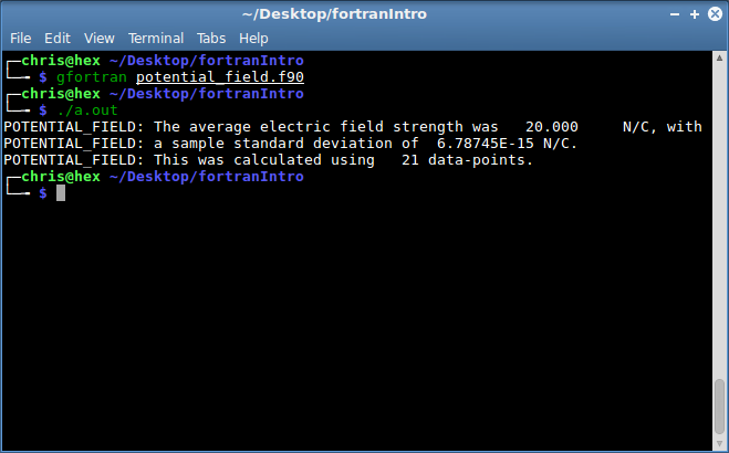
The output file out.dat should match this one. You should see an electric field that rounds to 20 NC^-1 everywhere. Don’t worry if your numbers vary from mine in the last few decimal places. The last decimal places of floating point values often vary from computer to computer and from compiler to compiler because of the finite levels of precision with which floating point numbers can be stored.

If your input data is contained in some file other than in.dat then you can run the program using the command ./a.out infile. If you want your output data to go to a file other than out.dat then run the program with the command ./a.out infile outfile.

You could also compile your program with the command gfortran -o potential_field potential_field.f90. This will produce an executable called potential_field. Had a different argument been placed after the -o flag then that would have been the name of the executable. The program would now be run using the command ./potential_field. Once again, you can optionally extra arguments specifying the input and output files.

Packaging Your Procedures

For a small, simple program like this it is easiest to keep everything in one file. However, as your program becomes larger, it will become desirable to put certain things into separate files. This prevents files from becoming overwhelmingly huge.⁶ It also means that if you want to reuse some of your procedures in other programs, it will be a lot easier to transfer them over. If you compile them correctly (not something we’ll get into here) then you won’t even need to transfer them—you can use the same “library” file for multiple programs.

In order to retain the compiler’s ability to know whether we are passing the correct arguments to a procedure we need to place that procedures in a “module”. Modules are a bit like programs, containing both variables and procedures (also “derived types,” in case you ever want to use them). However, unlike programs, they can not be run on their own; they just contain code to be used by other modules and programs. The basic syntax for our module is

MODULE tools
    IMPLICIT NONE

    !Variable declarations
    ! ...

CONTAINS
    ! Procedures
    ! ...

END MODULE tools

If your module does not contain any procedures then omit the CONTAINS statement.

To make a module’s contents available to a program (or another module) you place a USE statement followed by the module name at the very start of your program—before even the IMPLICIT NONE statement. In our case this means that our program starts with

PROGRAM potential_field
    USE tools
    IMPLICIT NONE
    ! ...

If you need to load multiple modules then you place additional USE statements at the start of the program, each on its own line. Take a look at the module and modified program to see what changes were made.

The main disadvantage of using modules (although it’s one that can be overcome with sufficient organization and/or appropriate software tools) is that it makes the compile process more complicated. It is important that module files are compiled before any files which use them. This is because, upon compiling the module into an “object file,” the compiler will produce a file ending in the extension .mod. This file contains information for the compiler about the contents of the module and which will need to read as it compiles anything that uses the module. Needless to say, if you have modules using other modules then things can get complicated.

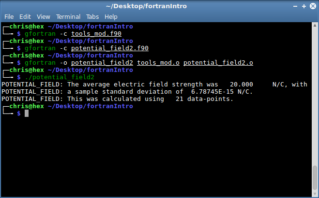
In this case we can compile like so:

gfortran -c tools_mod.f90
gfortran -c potential_field2.f90
gfortran -o potential_field2 tools_mod.o potential_field2.o

Aside from the change in the name of the executable, the program can be run just as before.

Summing Up

There you have it. You’ve now seen how various features in Fortran work and seen an example of a working program. Although this was a lot of information all at once, Fortran really isn’t a hard language to learn. The syntax is intuitive and the modern version comes with enough features to be useful but not so many as be overwhelming. Don’t feel bad if you’ve forgotten some of the syntax that I’ve gone over—even experienced programmers will occasionally have to look something up. Hopefully now you’ll feel ready to try writing a program of your own in Fortran and begin learning the language’s capabilities and limitations in the best way possible: through experience.

Useful Resources

There are plenty of features in Fortran which I have not mentioned. If you want to learn more about them, some useful links are given below:

• Fortran 95 language features: A Wikipedia article which gives a good overview of the various capabilities of Fortran 95. I regularly use this as a reference when I forget some syntax.
• Mistakes in Fortran 90 Programs that Might Surprise You: A webpage describing some of the more obscure behaviour of Fortran. It’s good to be familiar with what these are. If your program is behaving strangely, these are all good things to check for.
• Fortran Formats: Some information on how format strings can be used to specify output (and, in principle, input) in Fortran.
• The GNU Fortran Compiler: The manual for gfortran, the main free compiler. In my opinion it is the best documented compiler out there. Particularly useful is its list of intrinsic functions and subroutines, which comes with information and, usually, an example for each one.
• The New Features of Fortran 2003: A PDF providing an introduction to what’s new in the Fortran 2003 standard. Note that not all features are yet supported by all compilers.
• The New Features of Fortran 2008: A PDF providing an introduction to what’s new in the Fortran 2008 standard. Note that not all features are yet supported by all compilers.